Tests for the univ() function - Exponential Distribution

Ivan Jacob Agaloos Pesigan

2020-07-17

library(testthat)
library(MASS)
library(jeksterslabRdata)
context("Test univ Exponential Distribution.")

Univariate Data Generation - Exponential Distribution

Sample Size and Monte Carlo replications

Sample Size and Monte Carlo Replications

Variable	Description	Notation	Values
n	Sample size.	\(n\)	1000
R	Monte Carlo replications.	\(R\)	1000

Population Parameters

Population Parameters

Variable	Description	Notation	Values
lambda	Population rate.	\(\lambda\)	1
mu	Population mean.	\(\mu\)	1
sigma2	Population variance.	\(\sigma^2\)	1
sigma	Population standard deviation.	\(\sigma\)	1

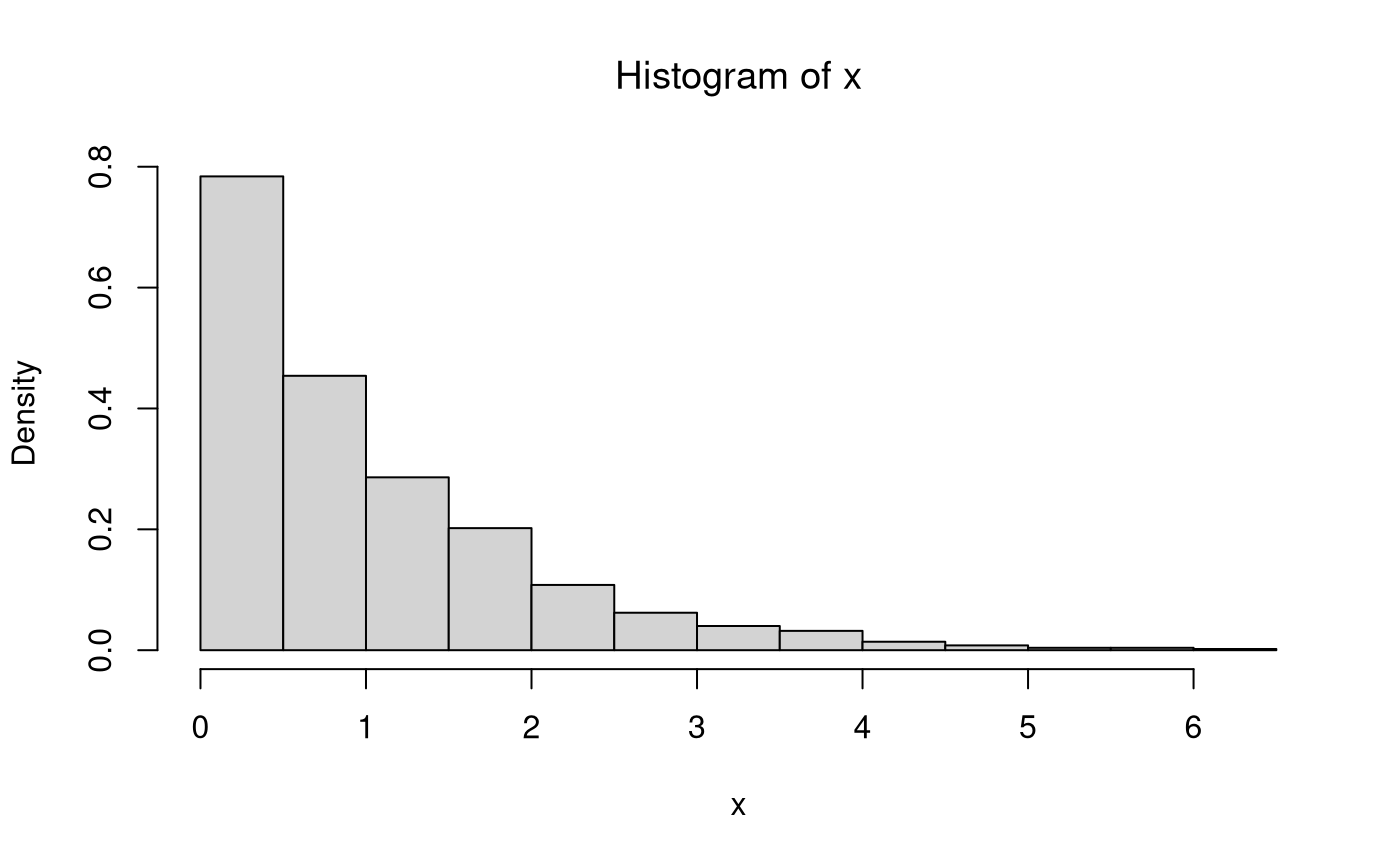
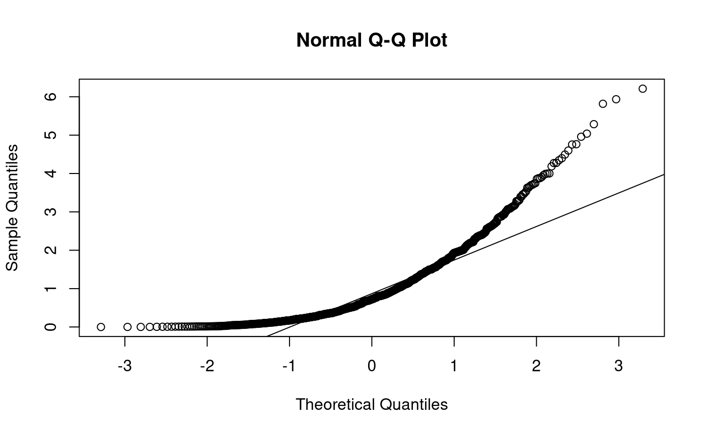
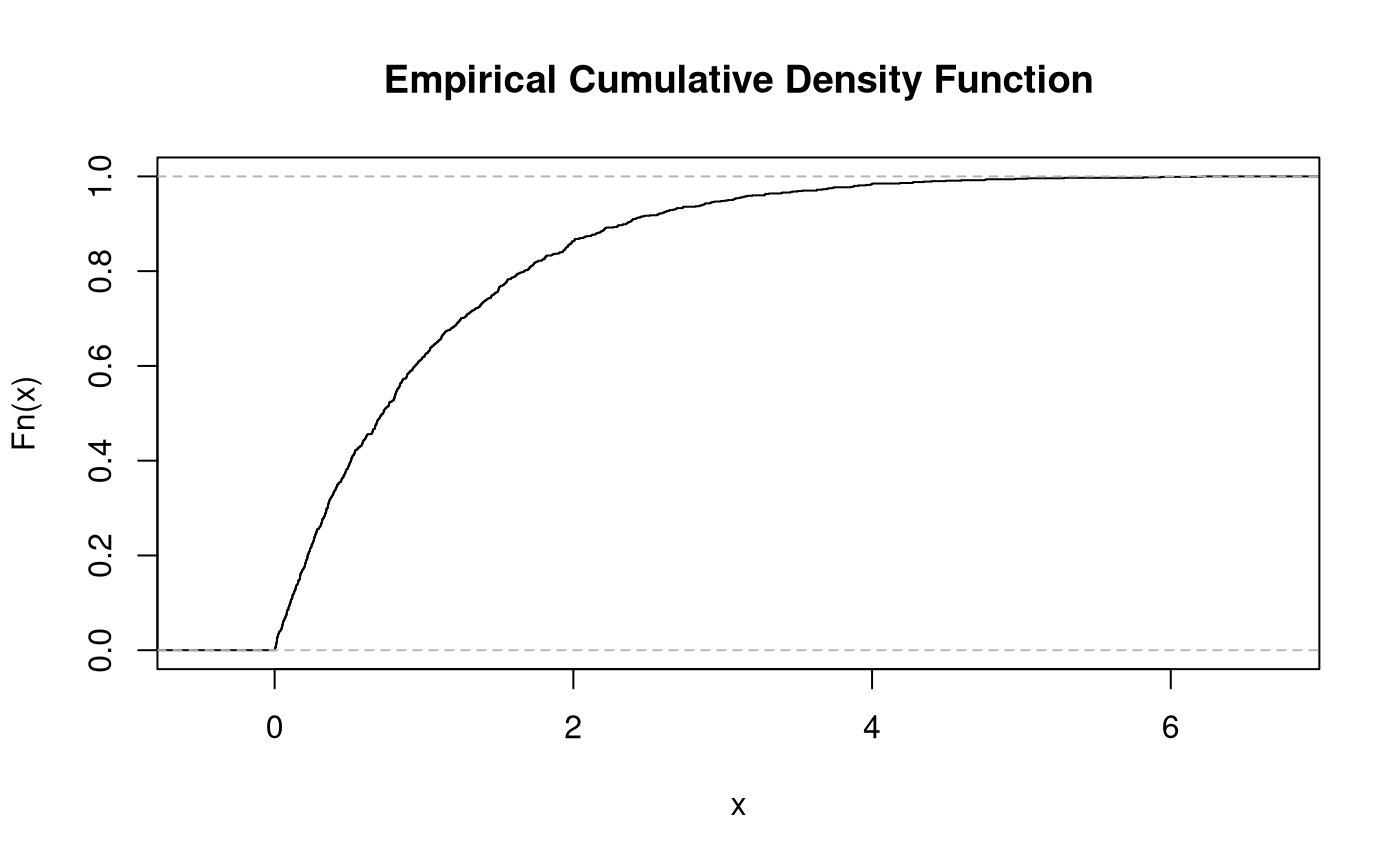
Sample Data

\[\begin{equation} X \sim \mathrm{exp} \left( \lambda \right) %(\#eq:dist-exp-X-r) \end{equation}\]

The random variable \(X\) takes on the value \(x\) for each observation \(\omega \in \Omega\).

• \(\omega\) refers to units or observations
• \(\Omega\) refers to the collection of all units, that is, a set of possible outcomes or the sample space contained in the set \(S\).

A random variable acts as a function, inasmuch as, it maps each observation \(\omega \in \Omega\) to a value \(x\).

\[\begin{equation} x = X \left( \omega \right) %(\#eq:dist-random-variable-1) \end{equation}\]

\[\begin{equation} \mathbf{x} = \begin{bmatrix} x_1 = X \left( \omega_1 \right) \\ x_2 = X \left( \omega_2 \right) \\ x_3 = X \left( \omega_3 \right) \\ x_i = X \left( \omega_i \right) \\ \vdots \\ x_n = X \left( \omega_n \right) \end{bmatrix}, \\ i = \left\{ 1, 2, 3, \dots, n \right\} %(\#eq:dist-random-variable-2) \end{equation}\]

Monte Carlo Simulation

Monte Carlo Simulation Results

Variable	Description	Notation	Values	Mean of estimates	Variance of estimates	Standard deviation of estimates
lambda	Population rate.	\(\lambda\)	1	1.0002573	0.0009942	0.0315303
mu	Population mean.	\(\mu\)	1	1.0007347	0.0009943	0.0315320
sigma2	Population variance.	\(\sigma^2\)	1	0.9994966	0.0081077	0.0900426
sigma	Population standard deviation.	\(\sigma\)	1	0.9987466	0.0020038	0.0447637

Sampling Distribution of Sample Lambdas

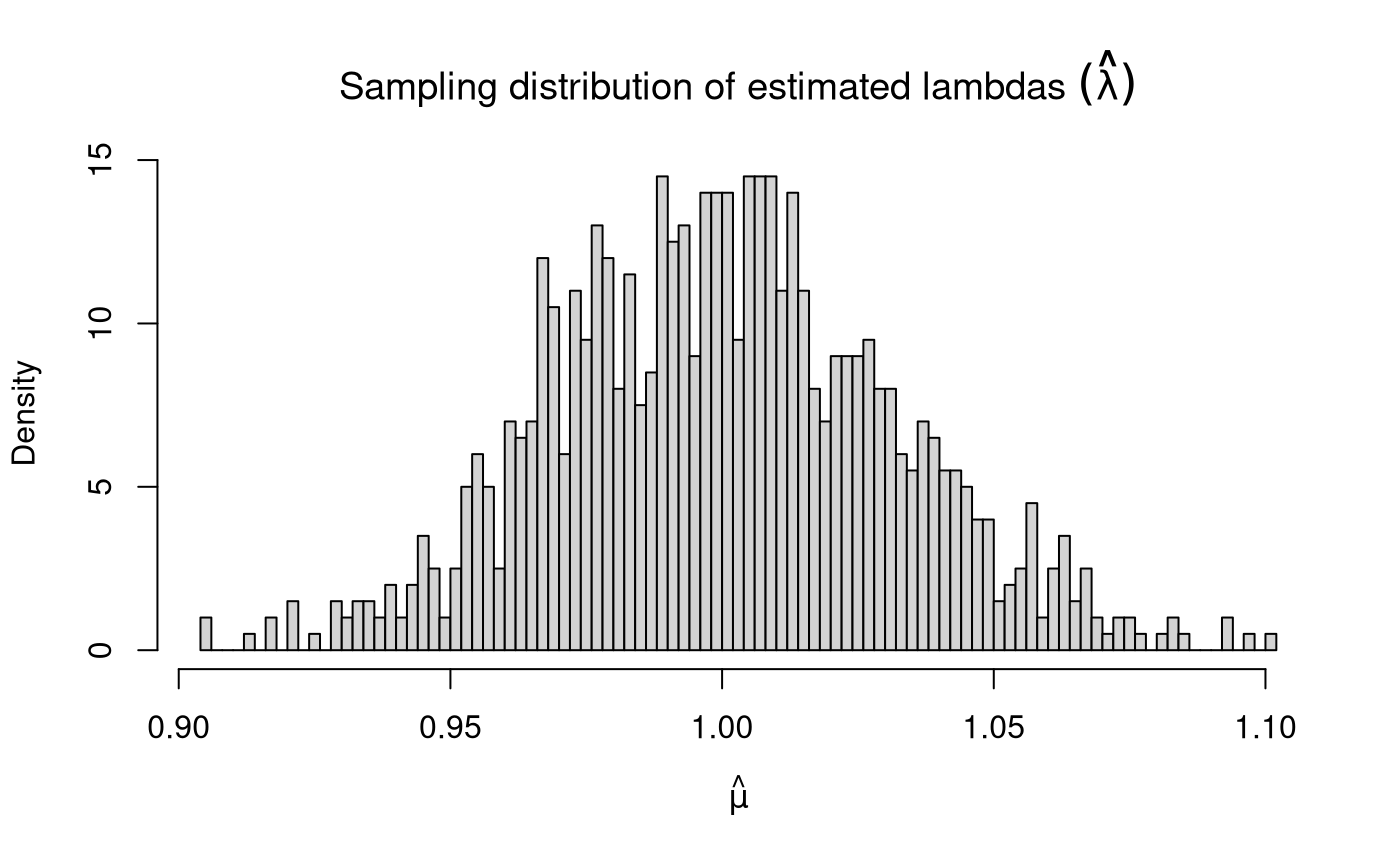
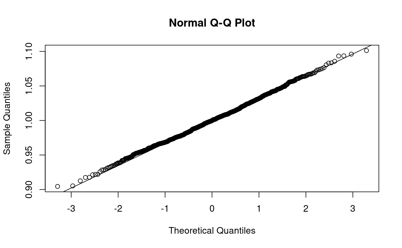
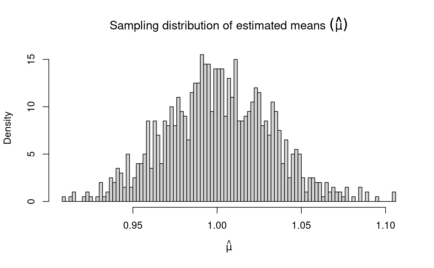
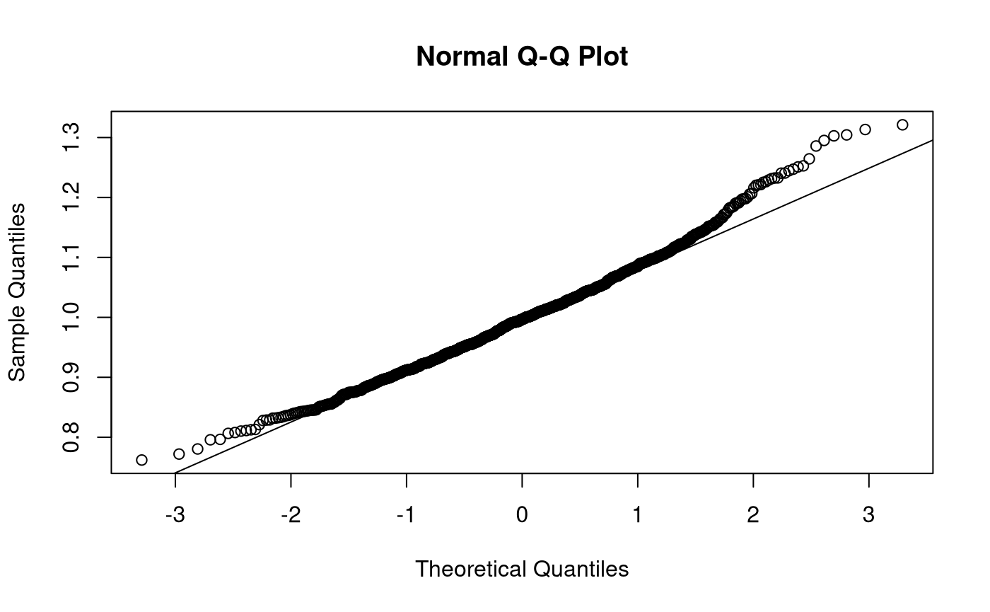
Sampling Distribution of Sample Means

\[\begin{equation} \hat{\mu} \sim \mathcal{N} \left( \mu, \frac{\sigma^2}{n} \right) %(\#eq:dist-sampling-dist-mean) \end{equation}\]

\[\begin{equation} \mathbb{E} \left[ \hat{\mu} \right] = \mu %(\#eq:dist-sampling-dist-mean-expected-value) \end{equation}\]

\[\begin{equation} \mathrm{Var} \left( \hat{\mu} \right) = \frac{\sigma^2}{n} %(\#eq:dist-sampling-dist-mean-var) \end{equation}\]

\[\begin{equation} \mathrm{se} \left( \hat{\mu} \right) = \frac{\sigma}{\sqrt{n}} %(\#eq:dist-sampling-dist-mean-se) \end{equation}\]

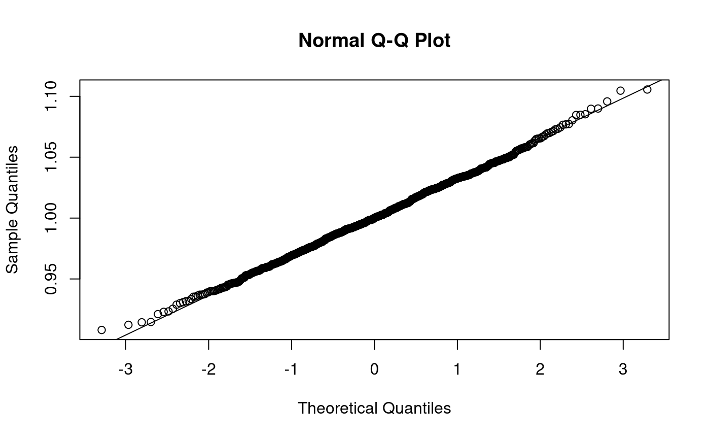
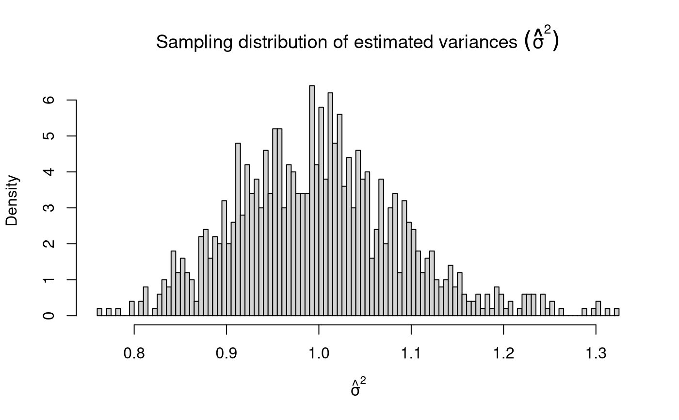
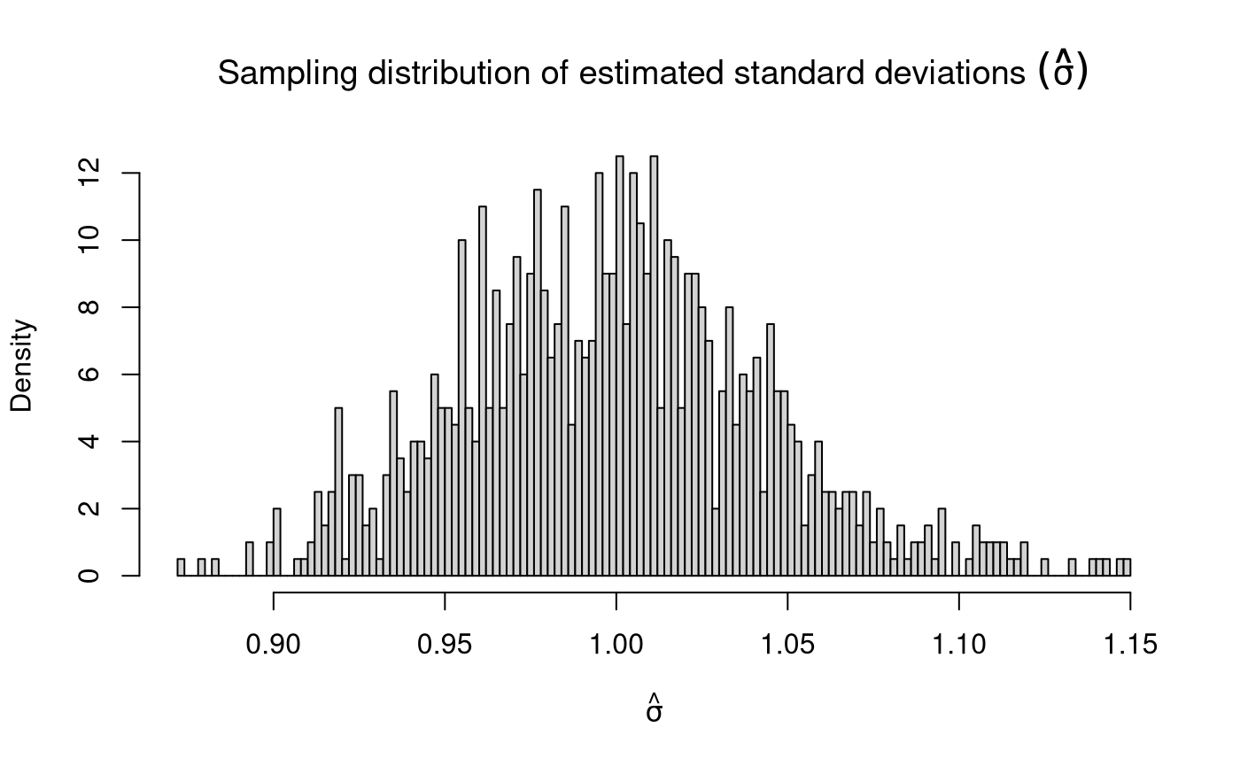
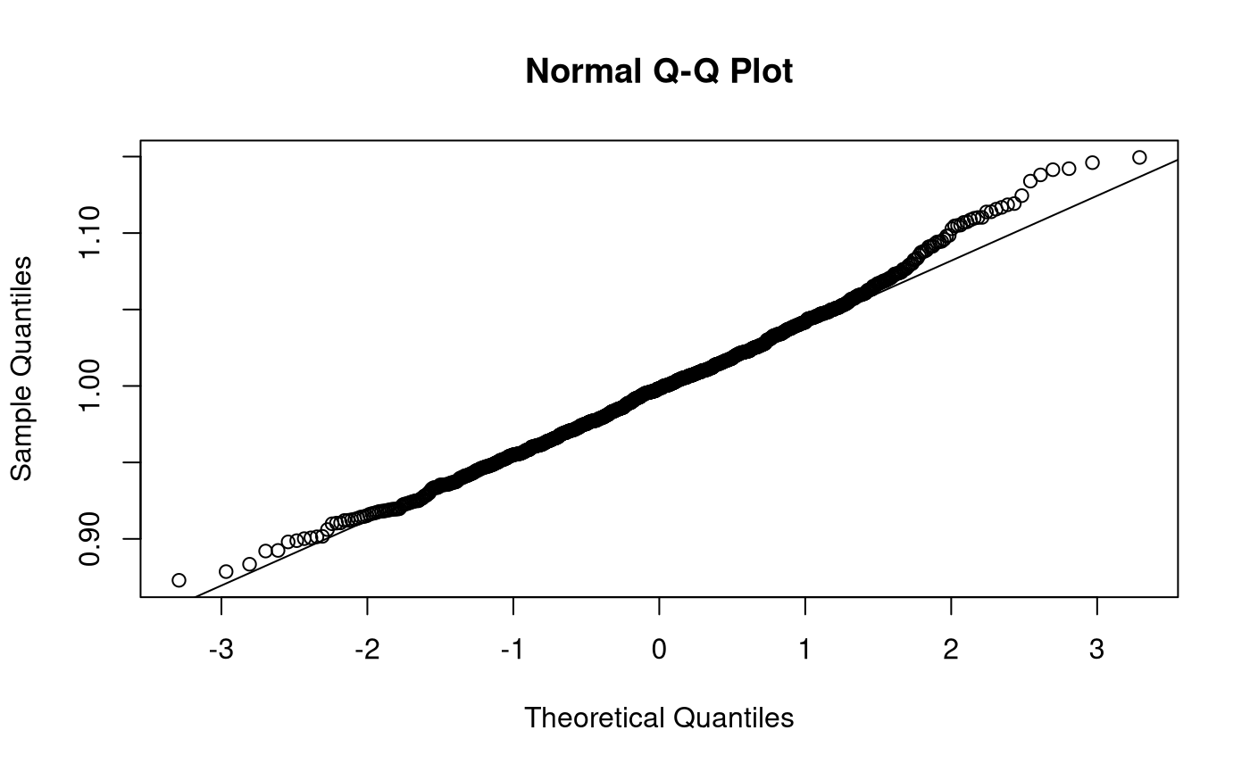
Sampling Distribution of Sample Variances

\[\begin{equation} \hat{\sigma}^2 \sim \chi^2 \left( k = n - 1 \right), \quad \text{when} \quad X \sim \left( \mu, \sigma^2 \right) %(\#eq:dist-sampling-dist-var) \end{equation}\]

\[\begin{equation} \mathbb{E} \left[ \hat{\sigma}^2 \right] = \sigma^2 %(\#eq:dist-sampling-dist-var-expected-value) \end{equation}\]

\[\begin{equation} \mathrm{Var} \left( \hat{\sigma}^2 \right) = \frac{ \left( n - 1 \right) \hat{\sigma}^2 }{ \sigma^2 }, \quad \text{where} \quad X \sim \mathcal{N} \left( \mu, \sigma^2 \right) %(\#eq:dist-sampling-dist-var-var) \end{equation}\]

When \(X \sim \mathcal{N} \left( \mu, \sigma^2 \right)\), \(\mathrm{Var} \left( \hat{\sigma}^2 \right) \sim \chi^2 \left( k = n - 1 \right)\). As \(k\) tends to infinity, the distribution of \(\mathrm{Var} \left( \hat{\sigma}^2 \right)\) converges to normality. When the \(X\) is not normally distributed, the variance of the sampling distribution of the sample variances takes on a slightly different functional form. Increase in sample size, however large it may be, does not help in approximating the normal distribution.

test_that("expected values (means) of muhat, sigma2hat, sigmahat", {
  expect_equivalent(
    round(
      means,
      digits = 0
    ),
    c(
      lambda,
      mu,
      sigma2,
      sigma
    )
  )
})