Examples for the univ() function
Ivan Jacob Agaloos Pesigan
2020-07-17
Source:vignettes/examples/examples_univ.Rmd
examples_univ.Rmdlibrary(jeksterslabRdata)
Documentation
See univ() for more details.
Examples
Normal Distribution
Single Random Data Set
Run the function.
Explore the output.
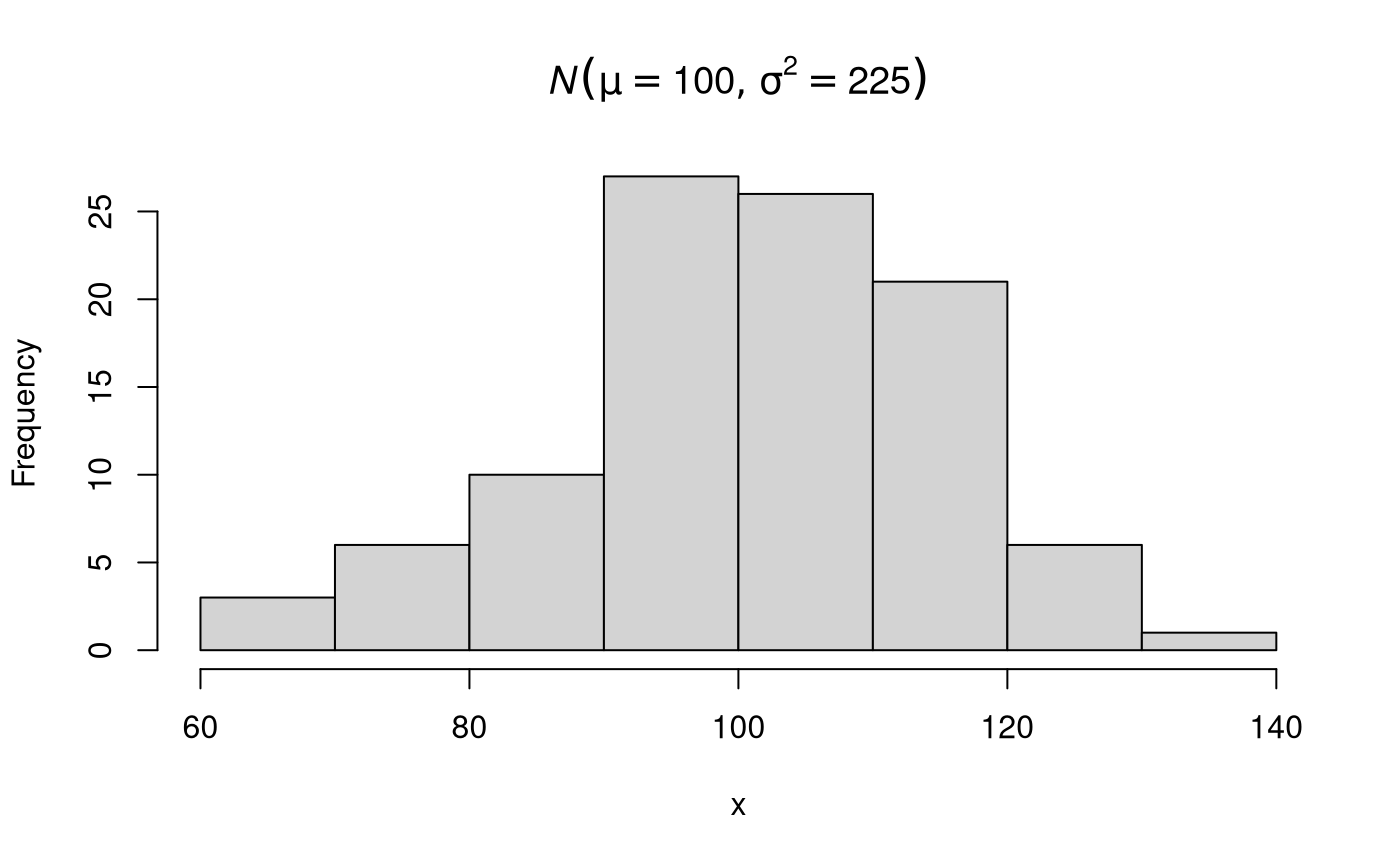
str(x, list.len = 6)
#>  num [1:100] 108 104.8 114.2 84.8 125.6 ...
hist(x, main = expression(italic(N)(list(mu == 100, sigma^2 == 225))))
Multiple Random Data Sets
Run the function.
Explore the output.
str(xstar, list.len = 6)
#> List of 100
#>  $ : num [1:100] 87.8 125.7 70.4 90.8 122.1 ...
#>  $ : num [1:100] 88.8 92.2 83 116.5 91.6 ...
#>  $ : num [1:100] 103.6 108 93.5 89.5 92.7 ...
#>  $ : num [1:100] 108 102 118 85 116 ...
#>  $ : num [1:100] 109.3 74 90.3 104.1 105.8 ...
#>  $ : num [1:100] 98.1 101.5 88.8 100.8 108.7 ...
#>   [list output truncated]
Bernoulli Distribution
Single Random Data Set
Run the function.
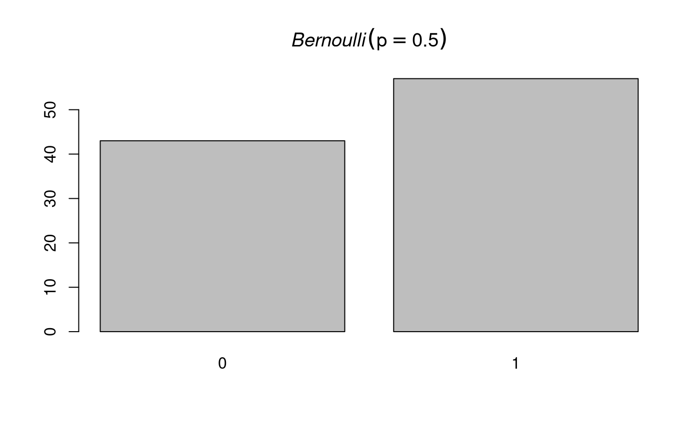
x <- univ(n = 100, rFUN = rbinom, size = 1, prob = 0.50)
Explore the output.
str(x, list.len = 6)
#>  int [1:100] 0 1 0 0 1 1 1 1 0 0 ...
barplot(table(x), main = expression(italic("Bernoulli")(p == 0.50)))
Multiple Random Data Sets
Run the function.
x <- univ(n = 100, rFUN = rbinom, size = 1, prob = 0.50, R = 100)
Explore the output.
str(xstar, list.len = 6)
#> List of 100
#>  $ : num [1:100] 87.8 125.7 70.4 90.8 122.1 ...
#>  $ : num [1:100] 88.8 92.2 83 116.5 91.6 ...
#>  $ : num [1:100] 103.6 108 93.5 89.5 92.7 ...
#>  $ : num [1:100] 108 102 118 85 116 ...
#>  $ : num [1:100] 109.3 74 90.3 104.1 105.8 ...
#>  $ : num [1:100] 98.1 101.5 88.8 100.8 108.7 ...
#>   [list output truncated]
Binomial Distribution
Single Random Data Set
Run the function.
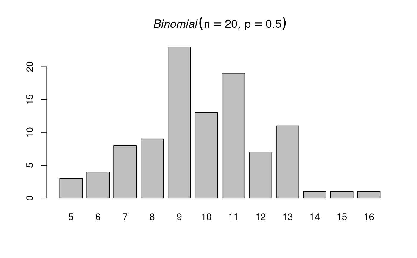
x <- univ(n = 100, rFUN = rbinom, size = 20, prob = 0.50)
Explore the output.
str(x, list.len = 6)
#>  int [1:100] 9 13 6 9 10 9 7 8 13 11 ...
barplot(table(x), main = expression(italic("Binomial")(list(n == 20, p == 0.50))))
Multiple Random Data Sets
Run the function.
x <- univ(n = 100, rFUN = rbinom, size = 20, prob = 0.50, R = 100)
Explore the output.
str(xstar, list.len = 6)
#> List of 100
#>  $ : num [1:100] 87.8 125.7 70.4 90.8 122.1 ...
#>  $ : num [1:100] 88.8 92.2 83 116.5 91.6 ...
#>  $ : num [1:100] 103.6 108 93.5 89.5 92.7 ...
#>  $ : num [1:100] 108 102 118 85 116 ...
#>  $ : num [1:100] 109.3 74 90.3 104.1 105.8 ...
#>  $ : num [1:100] 98.1 101.5 88.8 100.8 108.7 ...
#>   [list output truncated]
Exponential Distribution
Single Random Data Set
Run the function.
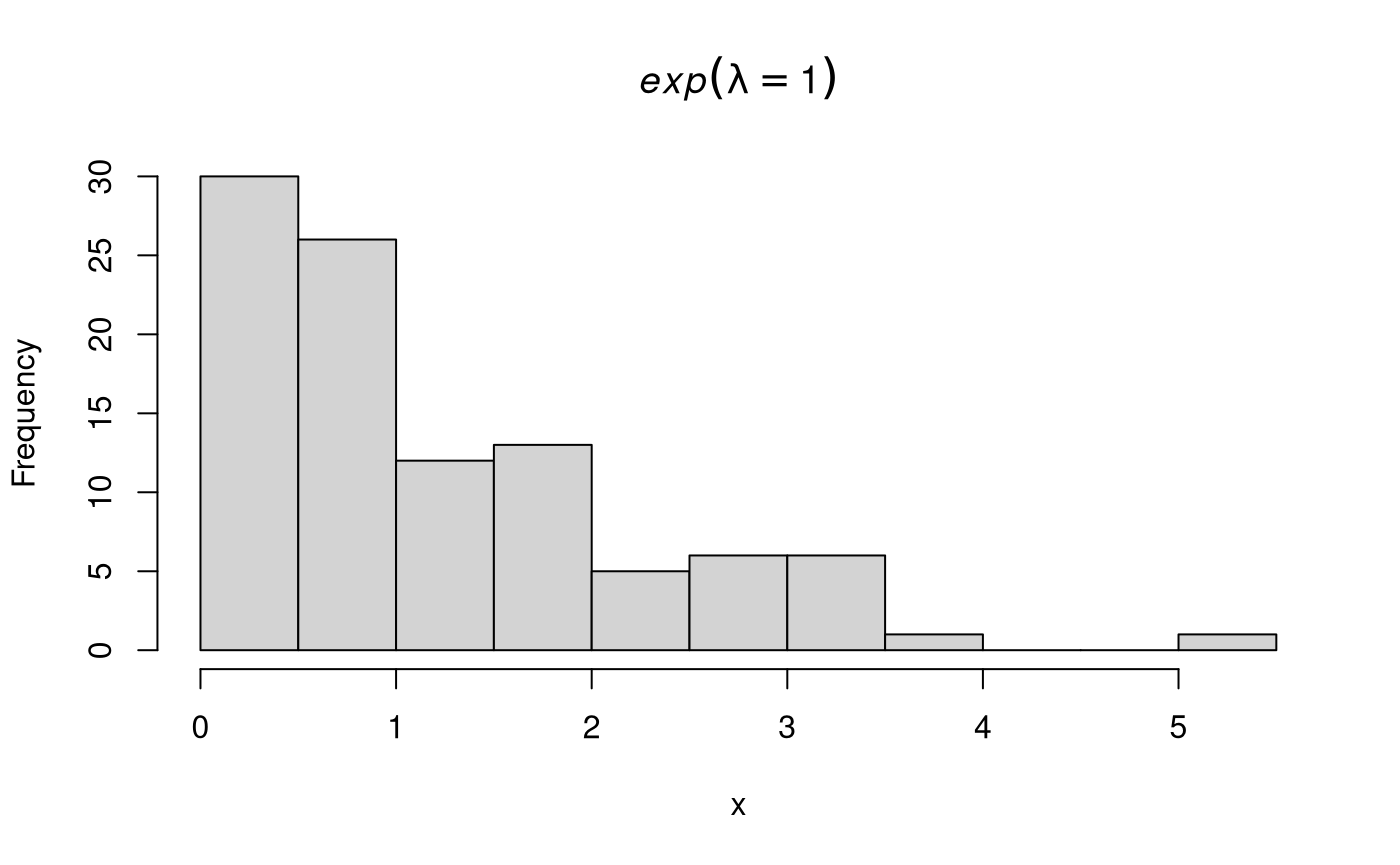
x <- univ(n = 100, rFUN = rexp, rate = 1)
Explore the output.
str(x, list.len = 6)
#>  num [1:100] 0.883 1.319 0.614 0.254 2.704 ...
hist(x, main = expression(italic(exp)(lambda == 1)))
Multiple Random Data Sets
Run the function.
xstar <- univ(n = 100, rFUN = rexp, rate = 1, R = 100)
Explore the output.
str(xstar, list.len = 6)
#> List of 100
#>  $ : num [1:100] 0.2937 0.2199 0.4766 1.6492 0.0696 ...
#>  $ : num [1:100] 1.32 3.991 0.584 1.001 1.94 ...
#>  $ : num [1:100] 0.038 0.432 1.195 0.168 0.21 ...
#>  $ : num [1:100] 0.261 0.585 0.616 0.832 3.581 ...
#>  $ : num [1:100] 0.0944 0.6773 0.7697 0.2163 0.3733 ...
#>  $ : num [1:100] 0.2226 1.4949 0.8644 0.0117 1.5858 ...
#>   [list output truncated]