Calculates jackknife estimates.
jack_hat(
  thetahatstarjack,
  thetahat,
  alpha = c(0.001, 0.01, 0.05),
  eval = FALSE,
  theta = 0
)
Arguments
| thetahatstarjack | Numeric vector.
Jackknife sampling distribution,
that is,
the sampling distribution of |
|---|---|
| thetahat | Numeric. Parameter estimate \( \left( \hat{ \theta } \right) \) from the original sample data. |
| alpha | Numeric vector.
Significance level
\(\left( \alpha \right)\) .
By default,
|
| eval | Logical.
Evaluate confidence intervals using
|
| theta | Numeric. Population parameter \( \left( \theta \right) \). |
Value
Returns a list with the following elements:
Jackknife estimates.
Pseudo-values.
Confidence intervals using pseudo-values.
The first list element hat contains the following:
Mean of thetahatstarjack \(\left( \hat{\theta}_{\left( \cdot \right) } \right)\).
Jackknife estimate of bias \(\left( \widehat{\mathrm{bias}}_{\mathrm{jack}} \left( \theta \right) \right)\).
Jackknife estimate of standard error \(\left( \widehat{\mathrm{se}}_{\mathrm{jack}} \left( \hat{\theta} \right) \right)\).
Bias-corrected jackknife estimate \(\left( \hat{\theta}_{\mathrm{jack}} \right)\).
Details
The jackknife estimate of bias is given by $$ \widehat{ \mathrm{ bias } }_{ \mathrm{ jack } } \left( \theta \right) = \left( n - 1 \right) \left( \hat{ \theta }_{ \left( \cdot \right) } - \hat{ \theta } \right) $$
where
$$ \hat{ \theta }_{ \left( \cdot \right) } = \frac{ 1 } { n } \sum_{ i = 1 }^{ n } \hat{ \theta }_{ \left( i \right) } . $$
The jackknife estimate of standard error is given by
$$ \widehat{ \mathrm{ se } }_{ \mathrm{ jack } } \left( \hat{ \theta } \right) = \sqrt{ \frac{ n - 1 } { n } \sum_{ i = 1 }^{ n } \left( \hat{ \theta }_{ \left( i \right) } - \hat{ \theta }_{ \left( \cdot \right) } \right)^2 } . $$
The bias-corrected jackknife estimate is given by
$$ \hat{ \theta }_{ \mathrm{ jack } } = \hat{ \theta } - \hat{ \mathrm{ bias } }_{ \mathrm{ jack } } \left( \theta \right) = n \hat{ \theta } - \left( n - 1 \right) \hat{ \theta }_{ \left( \cdot \right) } . $$
Pseudo-values can be computed using
$$ \tilde{ \theta }_{ i } = n \hat{ \theta } - \left( n - 1 \right) \hat{ \theta }_{ \left( i \right) } . $$
The standard error can be estimated using the pseudo-values
$$ \widehat{ \mathrm{ se } }_{ \mathrm{ jack } } \left( \tilde{ \theta } \right) = \sqrt{ \sum_{ i = 1 }^{ n } \frac{ \left( \tilde{ \theta }_{ i } - \tilde{ \theta } \right)^2 } { \left( n - 1 \right) n } } $$
where
$$ \tilde{ \theta } = \frac{ 1 } { n } \sum_{ i = 1 }^{ n } \tilde{ \theta }_{ i } . $$
An interval can be generated using
$$ \tilde{ \theta } \pm t_{ \frac{ \alpha } { 2 } } \times \widehat{ \mathrm{ se } }_{ \mathrm{ jack } } \left( \tilde{ \theta } \right) $$ with degrees of freedom \( \nu = n - 1 \) .
References
Wikipedia: Jackknife resampling
See also
Other jackknife functions:
jack()
Examples
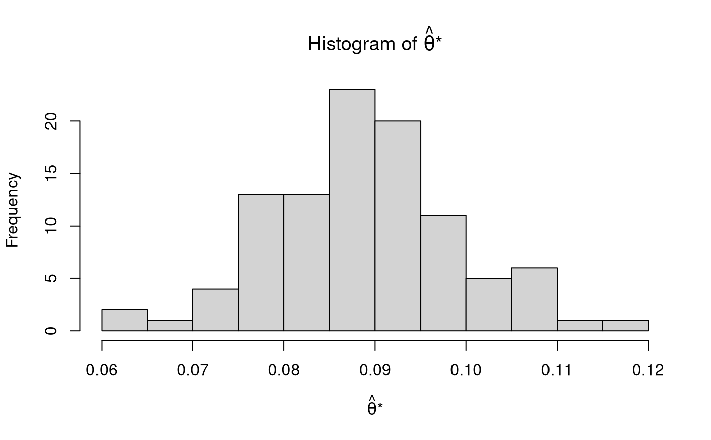
n <- 100
x <- rnorm(n = n)
thetahat <- mean(x)
xstar <- jack(
  data = x
)
thetahatstarjack <- sapply(
  X = xstar,
  FUN = mean
)
str(xstar, list.len = 6)#> List of 100
#>  $ : num [1:99] 0.363 -1.3045 0.7378 1.8885 -0.0974 ...
#>  $ : num [1:99] 0.4682 -1.3045 0.7378 1.8885 -0.0974 ...
#>  $ : num [1:99] 0.4682 0.363 0.7378 1.8885 -0.0974 ...
#>  $ : num [1:99] 0.4682 0.363 -1.3045 1.8885 -0.0974 ...
#>  $ : num [1:99] 0.4682 0.363 -1.3045 0.7378 -0.0974 ...
#>  $ : num [1:99] 0.468 0.363 -1.305 0.738 1.889 ...
#>   [list output truncated]hist(
  thetahatstarjack,
  main = expression(
    paste(
      "Histogram of ",
      hat(theta),
      "*"
    )
  ),
  xlab = expression(
    paste(
      hat(theta),
      "*"
    )
  )
)jack_hat(
  thetahatstarjack = thetahatstarjack,
  thetahat = thetahat
)#> $hat
#>         mean         bias           se thetahatjack      mean_ps        se_ps
#> 8.884876e-02 0.000000e+00 1.518905e-16 8.884876e-02 8.884876e-02 1.015632e-01
#>
#> $ps
#>   [1]  0.46815442  0.36295126 -1.30454355  0.73777632  1.88850493 -0.09744510
#>   [7] -0.93584735 -0.01595031 -0.82678895 -1.51239965  0.93536319  0.17648861
#>  [13]  0.24368546  1.62354888  0.11203808 -0.13399701 -1.91008747 -0.27923724
#>  [19] -0.31344598  1.06730788  0.07003485 -0.63912332 -0.04996490 -0.25148344
#>  [25]  0.44479712  2.75541758  0.04653138  0.57770907  0.11819487 -1.91172049
#>  [31]  0.86208648 -0.24323674 -0.20608719  0.01917759  0.02956075  0.54982754
#>  [37] -2.27411486  2.68255718 -0.36122126  0.21335575  1.07434588 -0.66508825
#>  [43]  1.11395242 -0.24589641 -1.17756331 -0.97585062  1.06505732  0.13167063
#>  [49]  0.48862881 -1.69945057 -1.47073631  0.28415034  1.33732041  0.23669628
#>  [55]  1.31829338  0.52390979  0.60674805 -0.10993567  0.17218172 -0.09032729
#>  [61]  1.92434334  1.29839276  0.74879127  0.55622433 -0.54825726  1.11053489
#>  [67] -2.61233433 -0.15569378  0.43388979 -0.38195111  0.42418757  1.06310200
#>  [73]  1.04871262 -0.03810289  0.48614892  1.67288261 -0.35436116  0.94634789
#>  [79]  1.31682636 -0.29664002 -0.38721358 -0.78543266 -1.05673687 -0.79554143
#>  [85] -1.75627543 -0.69053790 -0.55854199 -0.53666333  0.22712713  0.97845492
#>  [91] -0.20888265 -1.39941046  0.25853729 -0.44179945  0.56859986  2.12685046
#>  [97]  0.42485844 -1.68428153  0.24940178  1.07283825
#>
#> $ci
#>  statistic          p         se    ci_0.05     ci_0.5     ci_2.5    ci_97.5
#>         NA         NA  0.1015632 -0.2556056 -0.1778973 -0.1126746  0.2903721
#>    ci_99.5   ci_99.95
#>  0.3555948  0.4333032
#>