Notes: Nonparametric Bootstrapping - Mediation • jeksterslabRboot

Random Variables

Population Model

\[\begin{equation} Y = \delta_Y + \tau^{\prime} X + \beta M + \varepsilon_{Y} \end{equation}\]

\[\begin{equation} M = \delta_M + \alpha X + \varepsilon_{M} \end{equation}\]

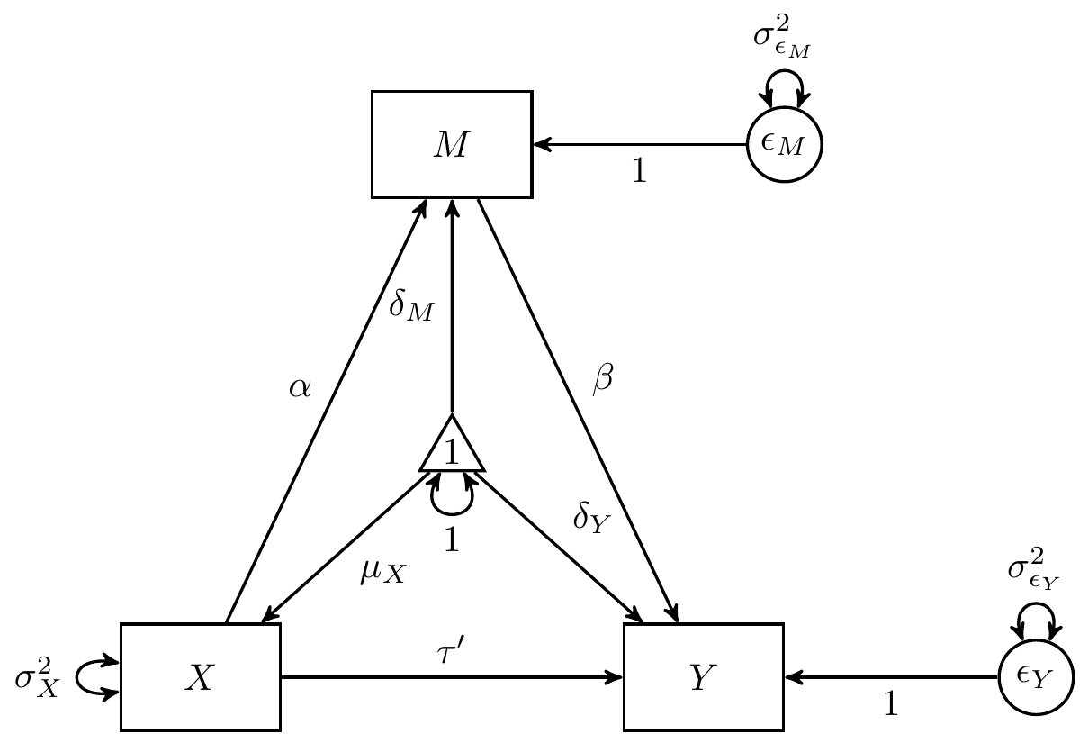
The Simple Mediation Model

Data Generating Function

\[\begin{equation} X, M, Y \sim \mathrm{MVN} \left[ \boldsymbol{\mu} \left( \boldsymbol{\theta} \right), \boldsymbol{\Sigma} \left( \boldsymbol{\theta} \right) \right] \end{equation}\]

\[\begin{equation} \boldsymbol{\mu} \left( \boldsymbol{\theta} \right) = \begin{bmatrix} \mu_X \\ \delta_M + \alpha \mu_X \\ \delta_Y + \tau^{\prime} \mu_X + \beta \delta_M + \alpha \beta \mu_X \end{bmatrix} \end{equation}\]

\[\begin{equation} \boldsymbol{\Sigma} \left( \boldsymbol{\theta} \right) = \begin{bmatrix} \sigma^{2}_{X} & \alpha \sigma_{X}^{2} & \alpha \beta \sigma_{X}^{2} + \tau^{\prime} \sigma_{X}^{2} \\ \alpha \sigma_{X}^{2} & \alpha^{2} \sigma_{X}^{2} + \sigma_{\varepsilon_{M}}^{2} & \alpha^{2} \beta \sigma_{X}^{2} + \alpha \tau^{\prime} \sigma_{X}^{2} + \beta \sigma_{\varepsilon_{M}}^{2} \\ \alpha \beta \sigma_{X}^{2} + \tau^{\prime} \sigma_{X}^{2} & \alpha^{2} \beta \sigma_{X}^{2} + \alpha \tau^{\prime} \sigma_{X}^{2} + \beta \sigma_{\varepsilon_{M}}^{2} & \beta^{2} \alpha^{2} \sigma_{X}^{2} + \beta^{2} \sigma_{\varepsilon_{M}}^{2} + 2 \alpha \beta \tau^{\prime} \sigma_{X}^{2} + \tau^{\prime} \sigma_{X}^{2} + \sigma_{\varepsilon_{Y}}^{2} \end{bmatrix} \end{equation}\]

Mean of \(X\) and Regression Intercepts
Variable	Description	Notation	Value
`muX`	Mean of \(X\).	\(\mu_X\)	70.18000
`deltaM`	Intercept of \(M\).	\(\delta_M\)	-20.70243
`deltaY`	Intercept of \(Y\).	\(\delta_Y\)	-12.71288

Regression Slopes
Variable	Description	Notation	Value
`alpha`	Regression slope of path from \(X\) to \(M\).	\(\alpha\)	0.3385926
`tauprime`	Regression slope of path from \(X\) to \(Y\).	\(\tau^{\prime}\)	0.2076475
`beta`	Regression slope of path from \(M\) to \(Y\).	\(\beta\)	0.4510391
`alphabeta`	Indirect effect.	\(\alpha \beta\)	0.1527185

Variance of \(X\) and Error Variances
Variable	Description	Notation	Value
`sigma2X`	Variance of \(X\).	\(\sigma^2_X\)	1.2934694
`sigma2epsilonM`	Error variance of \(\varepsilon_M\).	\(\sigma^2_{\varepsilon_{M}}\)	0.9296694
`sigma2epsilonY`	Error variance of \(\varepsilon_Y\).	\(\sigma^2_{\varepsilon_{Y}}\)	0.9310601

\(\boldsymbol{\mu} \left( \boldsymbol{\theta} \right)\) (`mutheta`)
	x
X	70.18
M	3.06
Y	3.24

\(\boldsymbol{\Sigma} \left( \boldsymbol{\theta} \right)\) (`Sigmatheta`)
	X	M	Y
X	1.2934694	0.4379592	0.4661224
M	0.4379592	1.0779592	0.5771429
Y	0.4661224	0.5771429	1.2881633

Sample Data

X <- as.data.frame(
  mvrnorm(
    n = n,
    Sigma = Sigmatheta,
    mu = mutheta
  )
)
str(X)
#> 'data.frame':    50 obs. of  3 variables:
#>  $ X: num  69.6 72.1 68.7 68.1 70.6 ...
#>  $ M: num  2.78 3.07 3.14 3.92 2.97 ...
#>  $ Y: num  1.678 4.526 -0.146 2.965 3.084 ...

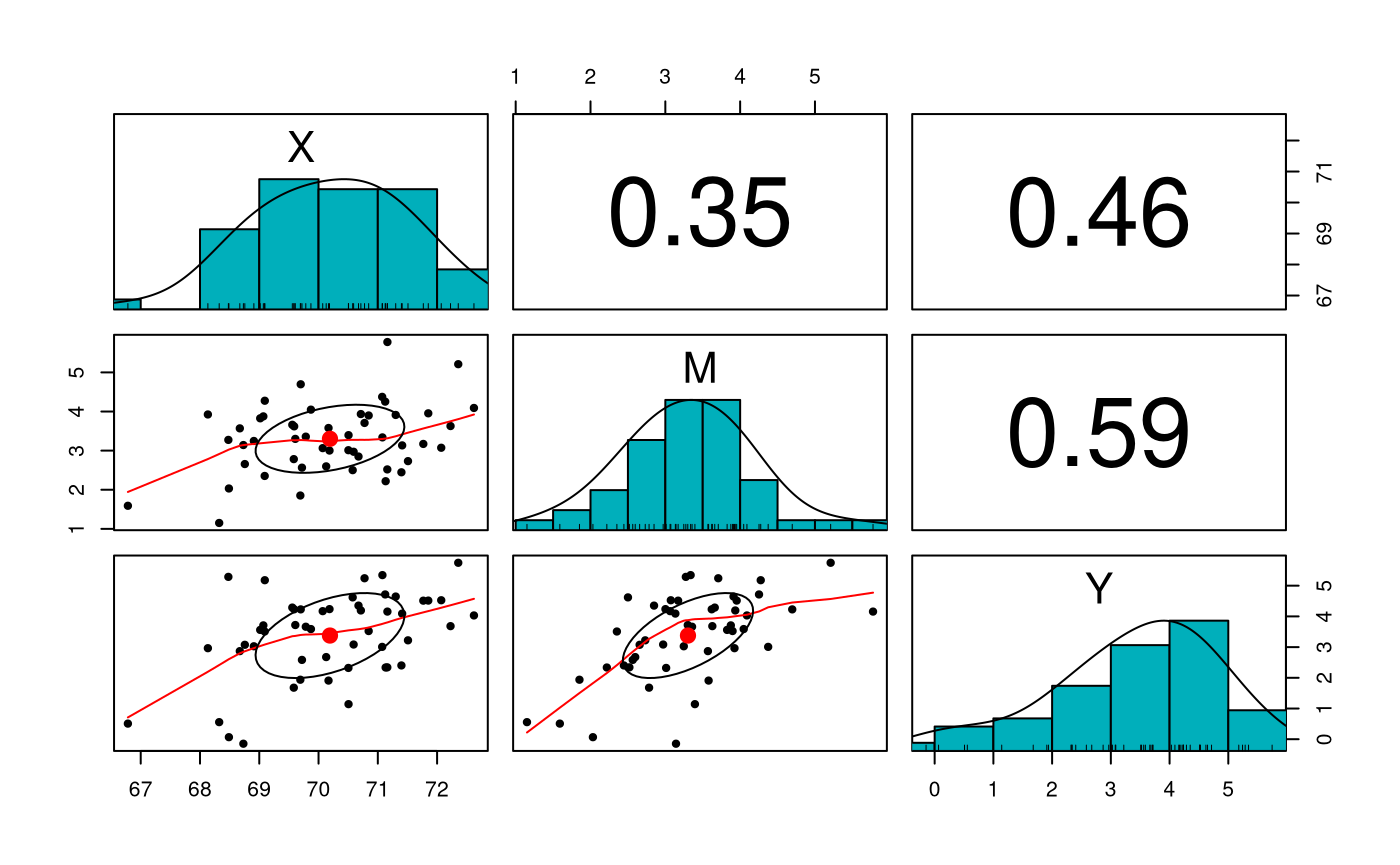
Sample Statistics

Estimated Mean Vector \(\boldsymbol{\hat{\mu}}\) (`muhat`)
	x
X	70.192661
M	3.302745
Y	3.376259

Estimated Variance-Covariance Matrix \(\boldsymbol{\hat{\Sigma}}\) (`Sigmahat`)
	X	M	Y
X	1.5763890	0.3874072	0.8057764
M	0.3874072	0.7581055	0.7052271
Y	0.8057764	0.7052271	1.9169666

model_01 <- lm(
  M ~ X,
  data = X
)
summary(model_01)
#> 
#> Call:
#> lm(formula = M ~ X, data = X)
#> 
#> Residuals:
#>      Min       1Q   Median       3Q      Max 
#> -1.69266 -0.60955  0.07842  0.49451  2.23514 
#> 
#> Coefficients:
#>             Estimate Std. Error t value Pr(>|t|)  
#> (Intercept) -13.9475     6.5710  -2.123   0.0390 *
#> X             0.2458     0.0936   2.626   0.0116 *
#> ---
#> Signif. codes:  0 '***' 0.001 '**' 0.01 '*' 0.05 '.' 0.1 ' ' 1
#> 
#> Residual standard error: 0.8226 on 48 degrees of freedom
#> Multiple R-squared:  0.1256, Adjusted R-squared:  0.1074 
#> F-statistic: 6.894 on 1 and 48 DF,  p-value: 0.01157
model_02 <- lm(
  Y ~ X + M,
  data = X
)
summary(model_02)
#> 
#> Call:
#> lm(formula = Y ~ X + M, data = X)
#> 
#> Residuals:
#>      Min       1Q   Median       3Q      Max 
#> -2.92809 -0.55738  0.02484  0.70308  2.48631 
#> 
#> Coefficients:
#>             Estimate Std. Error t value Pr(>|t|)    
#> (Intercept) -21.8313     9.0155  -2.422 0.019368 *  
#> X             0.3231     0.1313   2.461 0.017593 *  
#> M             0.7651     0.1893   4.041 0.000196 ***
#> ---
#> Signif. codes:  0 '***' 0.001 '**' 0.01 '*' 0.05 '.' 0.1 ' ' 1
#> 
#> Residual standard error: 1.079 on 47 degrees of freedom
#> Multiple R-squared:  0.4173, Adjusted R-squared:  0.3925 
#> F-statistic: 16.83 on 2 and 47 DF,  p-value: 3.076e-06

Sample Mean of \(X\) and Regression Intercepts (Parameter Estimates)
Variable	Description	Notation	Value
`muXhat`	Estimated mean of \(X\).	\(\hat{\mu_X}\)	70.19266
`deltaMhat`	Estimated intercept of \(M\).	\(\hat{\delta_M}\)	-13.94753
`deltaYhat`	Estimated intercept of \(Y\).	\(\hat{\delta_Y}\)	-21.83128

Sample Regression Slopes (Parameter Estimates)
Variable	Description	Notation	Value
`alphahat`	Estimated regression slope of path from \(X\) to \(M\).	\(\hat{\alpha}\)	0.2457561
`tauprimehat`	Estimated regression slope of path from \(X\) to \(Y\).	\(\hat{\tau}^{\prime}\)	0.3231180
`betahat`	Estimated regression slope of path from \(M\) to \(Y\).	\(\hat{\beta}\)	0.7651294
`alphahatbetahat`	Estimated indirect effect.	\(\hat{\alpha}\hat{\beta}\)	0.1880352

Variance of \(X\) and Error Variances
Variable	Description	Notation	Value
`sigma2Xhat`	Estimated variance of \(X\).	\(\hat{\sigma}^2_X\)	1.5763890
`sigma2epsilonMhat`	Estimated error variance of \(\varepsilon_M\).	\(\hat{\sigma}^2_{\varepsilon_{M}}\)	0.6767082
`sigma2epsilonYhat`	Estimated error variance of \(\varepsilon_Y\).	\(\hat{\sigma}^2_{\varepsilon_{Y}}\)	1.1645484

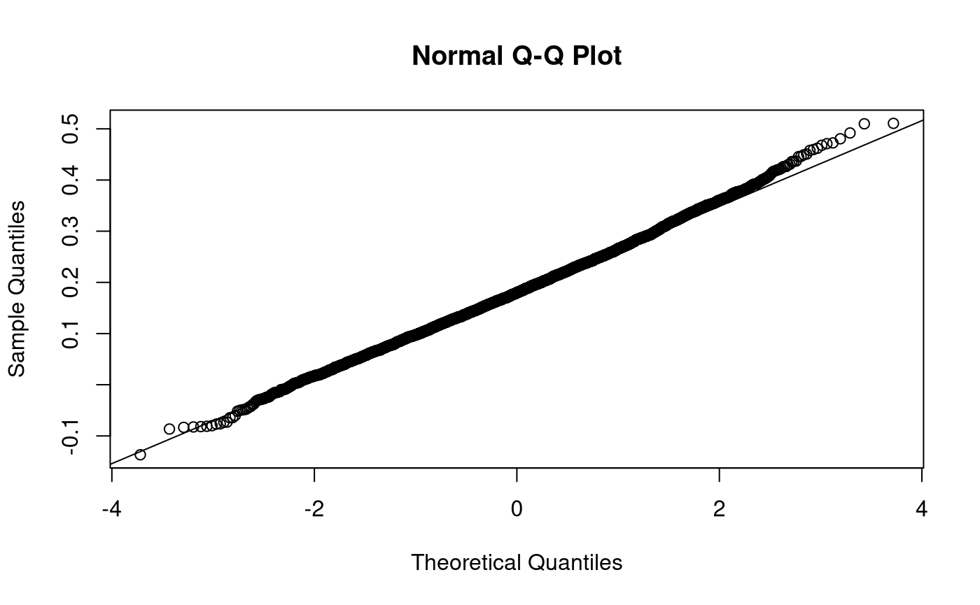
Nonparametric Bootstrapping

Bootstrap Samples

s <- function(X) {
  model_01 <- lm(
    M ~ X,
    data = X
  )
  model_02 <- lm(
    Y ~ X + M,
    data = X
  )
  coef(model_01)[2] * coef(model_02)[3]
}

Xstar <- nb(
  data = X,
  B = B
)

Bootstrap Sampling Distribution

thetahatstar <- sapply(
  X = Xstar,
  FUN = s
)

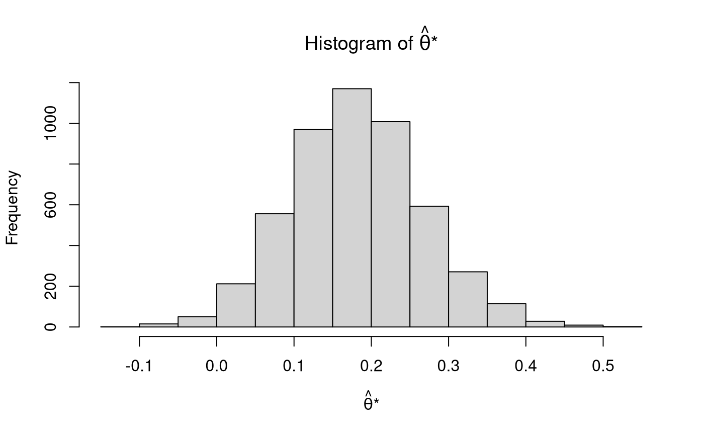
Estimated Bootstrap Standard Error

The estimated bootstrap standard error is given by

\[\begin{equation} \widehat{\mathrm{se}}_{\mathrm{B}} \left( \hat{\theta} \right) = \sqrt{ \frac{1}{B - 1} \sum_{b = 1}^{B} \left[ \hat{\theta}^{*} \left( b \right) - \hat{\theta}^{*} \left( \cdot \right) \right]^2 } = 0.0855372 \end{equation}\]

where

\[\begin{equation} \hat{\theta}^{*} \left( \cdot \right) = \frac{1}{B} \sum_{b = 1}^{B} \hat{\theta}^{*} \left( b \right) = 0.1819124 . \end{equation}\]

Note that \(\widehat{\mathrm{se}}_{\mathrm{B}} \left( \hat{\theta} \right)\) is the standard deviation of \(\boldsymbol{\hat{\theta}^{*}}\) and \(\hat{\theta}^{*} \left( \cdot \right)\) is the mean of \(\boldsymbol{\hat{\theta}^{*}}\) .

Nonparametric Bootstrapping Results
Variable	Description	Notation	Value
`B`	Number of bootstrap samples.	\(B\)	5000.0000000
`mean_thetahatstar`	Mean of \(B\) sample indirect effects.	\(\hat{\theta}^{} \left( \cdot \right) = \frac{1}{B} \sum_{b = 1}^{B} \hat{\theta}^{} \left( b \right)\)	0.1819124
`var_thetahatstar`	Variance of \(B\) sample indirect effects.	\(\widehat{\mathrm{Var}}_{\mathrm{B}} \left( \hat{\theta} \right) = \frac{1}{B - 1} \sum_{b = 1}^{B} \left[ \hat{\theta}^{} \left( b \right) - \hat{\theta}^{} \left( \cdot \right) \right]^2\)	0.0073166
`sd_thetahatstar`	Standard deviation of \(B\) sample indirect effects.	\(\widehat{\mathrm{se}}_{\mathrm{B}} \left( \hat{\theta} \right) = \sqrt{ \frac{1}{B - 1} \sum_{b = 1}^{B} \left[ \hat{\theta}^{} \left( b \right) - \hat{\theta}^{} \left( \cdot \right) \right]^2 }\)	0.0855372

Confidence Intervals

Confidence intervals can be constructed around \(\hat{\theta}\) . The functions pc(), bc(), and bca() from the jeksterslabRboot package can be used to construct confidence intervals using the default alphas of 0.001, 0.01, and 0.05. The confidence intervals can also be evaluated. Since we know the population parameter theta \(\left(\theta = \mu = 0.1527185 \right)\), we can check if our confidence intervals contain the population parameter.

See documentation for pc(), bc(), and bca() from the jeksterslabRboot package on how confidence intervals are constructed.

See documentation for zero_hit(), theta_hit(), len(), and shape() from the jeksterslabRboot package on how confidence intervals are evaluated.

pc_out <- pc(
  thetahatstar = thetahatstar,
  thetahat = thetahat,
  eval = TRUE,
  theta = theta
)
bc_out <- bc(
  thetahatstar = thetahatstar,
  thetahat = thetahat,
  eval = TRUE,
  theta = theta
)
bca_out <- bca(
  thetahatstar = thetahatstar,
  thetahat = thetahat,
  data = X,
  fitFUN = s,
  eval = TRUE,
  theta = theta
)

Confidence Intervals
	statistic	p	se	ci_0.05	ci_0.5	ci_2.5	ci_97.5	ci_99.5	ci_99.95	zero_hit_0.001	zero_hit_0.01	theta_hit_0.001	theta_hit_0.01	theta_hit_0.05	length_0.001	length_0.01	length_0.05	shape_0.001	shape_0.01	shape_0.05
pc	NA	NA	0.0855372	-0.0828897	-0.0312716	0.0193249	0.3558904	0.4195786	0.4862799	1	1	1	1	1	0.5691697	0.4508501	0.3365655	1.100839	1.055796	0.9949315
bc	NA	NA	0.0855372	-0.0813504	-0.0152843	0.0348956	0.3740522	0.4368202	0.5048616	1	1	1	1	1	0.5862121	0.4521045	0.3391567	1.176107	1.223616	1.2146883
bca	NA	NA	0.0855372	-0.0544361	0.0031244	0.0447128	0.3871218	0.4682649	0.5105386	1	0	1	1	1	0.5649747	0.4651405	0.3424091	1.330068	1.515485	1.3890815

Notes

References

Bollen, K. A., & Stine, R., (1990). Direct and indirect effects: Classical and bootstrap estimates of variability. Sociological Methodology, 20, 115-40. https://doi.org/10.2307/271084
Efron, B., & Tibshirani, R. J. (1993). An introduction to the bootstrap. New York, N.Y: Chapman & Hall.
MacKinnon, D. P. (2008). Introduction to statistical mediation analysis. New York: Lawrence Erlbaum Associates.
Shrout, P. E., & Bolger, N. (2002). Mediation in experimental and nonexperimental studies: New procedures and recommendations. Psychological Methods, 7, 422-445. https://doi.org/10.1037/1082-989X.7.4.422
Wikipedia: Bootstrapping (statistics)

Notes: Nonparametric Bootstrapping - Mediation

Ivan Jacob Agaloos Pesigan

2020-07-16