Residual Plots

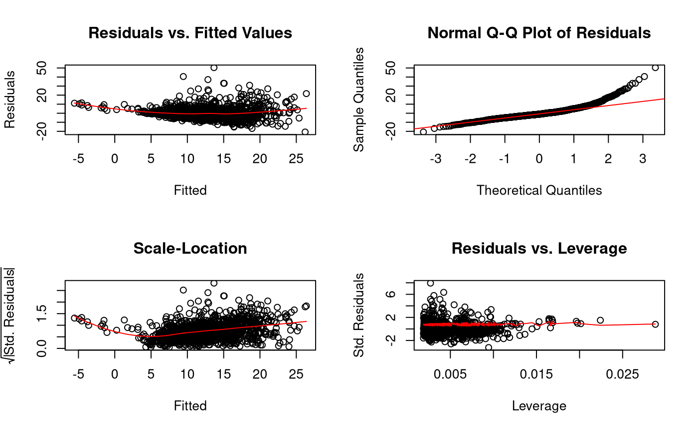
Displays a plot with four panels:

• residuals vs. fitted values

• normal qq plot of residuals

• scale location

• residuals vs. leverage

.residual.plot(yhat, epsilonhat, tepsilonhat, h)

Arguments

yhat	Numeric vector of length n or n by 1 numeric matrix. \(n \times 1\) vector of predicted values of \(\mathbf{y}\) \(\left( \mathbf{\hat{y}} \right)\).
epsilonhat	Numeric vector of length n or n by 1 numeric matrix. \(n \times 1\) vector of residuals \(\left( \boldsymbol{\hat{\epsilon}} \right)\).
tepsilonhat	Numeric vector of length n or n by 1 numeric matrix. \(n \times 1\) vector of studentized residuals.
h	Numeric vector of length n or n by 1 numeric matrix. \(n \times 1\) vector of leverage values.

Details

Based on the diagnostic plots in the car package.

See also

Other plotting functions: .scatter.plot()

Examples

model <- lm(
  wages ~ gender + race + union + education + experience,
  data = jeksterslabRdatarepo::wages
)
yhat <- as.vector(predict(model))
epsilonhat <- as.vector(residuals(model))
tepsilonhat <- as.vector(rstudent(model))
h <- as.vector(hatvalues(model))
.residual.plot(
  yhat = yhat, tepsilonhat = tepsilonhat,
  epsilonhat = epsilonhat, h = h
)