Tests: The Linear Regression Model
Ivan Jacob Agaloos Pesigan
2020-12-31
Source:vignettes/tests/test-linreg-estimation-linreg.Rmd
test-linreg-estimation-linreg.Rmd
# The Linear Regression Model {#linreg-estimation-linreg-example}Data
In this example, we are interested in predictors of wages. The regressor variables are gender, race, union membership, education, and work experience. The regressand variable is hourly wage in US dollars.
See jeksterslabRdatarepo::wages.matrix() for the data set used in this example.
X <- jeksterslabRdatarepo::wages.matrix[["X"]]
# age is removed
X <- X[, -ncol(X)]
y <- jeksterslabRdatarepo::wages.matrix[["y"]]
head(X)
#>      constant gender race union education experience
#> [1,]        1      1    0     0        12         20
#> [2,]        1      0    0     0         9          9
#> [3,]        1      0    0     0        16         15
#> [4,]        1      0    1     1        14         38
#> [5,]        1      1    1     0        16         19
#> [6,]        1      1    0     0        12          4
head(y)
#>      wages
#> [1,] 11.55
#> [2,]  5.00
#> [3,] 12.00
#> [4,]  7.00
#> [5,] 21.15
#> [6,]  6.92
jeksterslabRlinreg::linreg()
The jeksterslabRlinreg::linreg() function fits a linear regression model using X and y. In this example, X consists of a column of constants, gender, race, union membership, education, and work experience. and y consists of hourly wages in US dollars.
The output includes the following:
- Model assessment
- ANOVA table
- Table of regression coefficients with the following columns
- Regression coefficients
- Standard errors
- \(t\) statistic
- \(p\) value
- Standardized coefficients
- Confidence intervals (0.05, 0.5, 2.5, 97.5, 99.5, 99.95)
- Means and standard deviations
- Scatterplot matrix
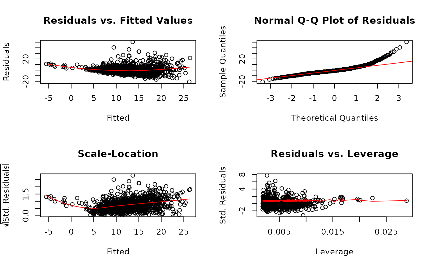
- Residual plots
Using Unbiased Standard Errors
linreg(
  X = X,
  y = y
)
#>
#> Model Assessment:
#>                   Value
#> RSS            54342.54
#> MSE               42.16
#> RMSE               6.49
#> R-squared          0.32
#> Adj. R-squared     0.32
#>
#> ANOVA Table:
#>         df       SS         MS        F             p
#> Model    5 25967.28 5193.45611 122.6149 3.453144e-106
#> Error 1283 54342.54   42.35584       NA            NA
#> Total 1288 80309.82         NA       NA            NA
#>
#> Coefficients:
#>                  coef         se         t            p
#> Intercept  -7.1833382 1.01578786 -7.071691 2.508276e-12
#> gender     -3.0748755 0.36461621 -8.433184 8.939416e-17
#> race       -1.5653133 0.50918754 -3.074139 2.155664e-03
#> union       1.0959758 0.50607809  2.165626 3.052356e-02
#> education   1.3703010 0.06590421 20.792312 5.507605e-83
#> experience  0.1666065 0.01604756 10.382050 2.659960e-24
#>
#> Standardized Coefficients:
#> Yuan and Chan 2011 standard errors are used.
#>                   coef         se         t            p
#> gender     -0.19477502 0.02282716 -8.532598 3.979462e-17
#> race       -0.07135673 0.02317122 -3.079541 2.117236e-03
#> union       0.05077872 0.02342286  2.167913 3.034867e-02
#> education   0.48829962 0.02113537 23.103429 5.007598e-99
#> experience  0.24607631 0.02330714 10.557981 4.800438e-25
#>
#> Confidence Intervals - Regression Coefficients:
#>                ci_0.05     ci_0.5     ci_2.5    ci_97.5    ci_99.5   ci_99.95
#> Intercept  -10.5335348 -9.8037324 -9.1761258 -5.1905507 -4.5629441 -3.8331417
#> gender      -4.2774257 -4.0154638 -3.7901849 -2.3595660 -2.1342872 -1.8723252
#> race        -3.2446781 -2.8788475 -2.5642449 -0.5663817 -0.2517792  0.1140514
#> union       -0.5731336 -0.2095371  0.1031443  2.0888072  2.4014886  2.7650852
#> education    1.1529406  1.2002901  1.2410091  1.4995928  1.5403119  1.5876614
#> experience   0.1136797  0.1252092  0.1351242  0.1980889  0.2080039  0.2195334
#>
#> Confidence Intervals - Standardized Slopes:
#>                ci_0.05       ci_0.5       ci_2.5     ci_97.5    ci_99.5
#> gender     -0.27006189 -0.253661495 -0.239557685 -0.14999235 -0.1358885
#> race       -0.14777833 -0.131130752 -0.116814367 -0.02589909 -0.0115827
#> union      -0.02647282 -0.009644448  0.004827412  0.09673002  0.1112019
#> education   0.41859249  0.433777402  0.446835936  0.52976331  0.5428218
#> experience  0.16920643  0.185951662  0.200352024  0.29180059  0.3062010
#>               ci_99.95
#> gender     -0.11948815
#> race        0.00506488
#> union       0.12803026
#> education   0.55800676
#> experience  0.32294619
#>
#> Means and Standard Deviations:
#>                  Mean         SD
#> wages      12.3658495  7.8963503
#> gender      0.4972847  0.5001867
#> race        0.1528317  0.3599648
#> union       0.1590380  0.3658535
#> education  13.1450737  2.8138234
#> experience 18.7897595 11.6628366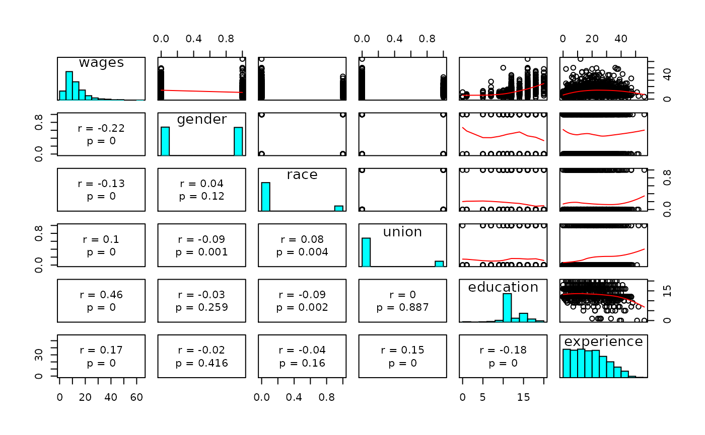

Using Biased Standard Errors
linreg(
  X = X,
  y = y,
  sehatbetahattype = "biased"
)
#>
#> Model Assessment:
#>                   Value
#> RSS            54342.54
#> MSE               42.16
#> RMSE               6.49
#> R-squared          0.32
#> Adj. R-squared     0.32
#>
#> ANOVA Table:
#>         df       SS         MS        F             p
#> Model    5 25967.28 5193.45611 122.6149 3.453144e-106
#> Error 1283 54342.54   42.35584       NA            NA
#> Total 1288 80309.82         NA       NA            NA
#>
#> Coefficients:
#> Biased standard errors are used.
#>                  coef         se         t            p
#> Intercept  -7.1833382 1.01342097 -7.088208 2.236468e-12
#> gender     -3.0748755 0.36376661 -8.452880 7.620029e-17
#> race       -1.5653133 0.50800108 -3.081319 2.104728e-03
#> union       1.0959758 0.50489888  2.170684 3.013798e-02
#> education   1.3703010 0.06575065 20.840873 2.582448e-83
#> experience  0.1666065 0.01601016 10.406297 2.103790e-24
#>
#> Standardized Coefficients:
#> Yuan and Chan 2011 standard errors are used.
#>                   coef         se         t            p
#> gender     -0.19477502 0.02282716 -8.532598 3.979462e-17
#> race       -0.07135673 0.02317122 -3.079541 2.117236e-03
#> union       0.05077872 0.02342286  2.167913 3.034867e-02
#> education   0.48829962 0.02113537 23.103429 5.007598e-99
#> experience  0.24607631 0.02330714 10.557981 4.800438e-25
#>
#> Confidence Intervals - Regression Coefficients:
#>                ci_0.05     ci_0.5     ci_2.5    ci_97.5    ci_99.5   ci_99.95
#> Intercept  -10.5257285 -9.7976266 -9.1714824 -5.1951941 -4.5690499 -3.8409480
#> gender      -4.2746237 -4.0132721 -3.7885182 -2.3612328 -2.1364788 -1.8751273
#> race        -3.2407650 -2.8757868 -2.5619173 -0.5687093 -0.2548398  0.1101384
#> union       -0.5692445 -0.2064951  0.1054577  2.0864938  2.3984466  2.7611960
#> education    1.1534470  1.2006862  1.2413104  1.4992916  1.5399157  1.5871549
#> experience   0.1138030  0.1253056  0.1351976  0.1980155  0.2079074  0.2194101
#>
#> Confidence Intervals - Standardized Slopes:
#>                ci_0.05       ci_0.5       ci_2.5     ci_97.5    ci_99.5
#> gender     -0.27006189 -0.253661495 -0.239557685 -0.14999235 -0.1358885
#> race       -0.14777833 -0.131130752 -0.116814367 -0.02589909 -0.0115827
#> union      -0.02647282 -0.009644448  0.004827412  0.09673002  0.1112019
#> education   0.41859249  0.433777402  0.446835936  0.52976331  0.5428218
#> experience  0.16920643  0.185951662  0.200352024  0.29180059  0.3062010
#>               ci_99.95
#> gender     -0.11948815
#> race        0.00506488
#> union       0.12803026
#> education   0.55800676
#> experience  0.32294619
#>
#> Means and Standard Deviations:
#>                  Mean         SD
#> wages      12.3658495  7.8963503
#> gender      0.4972847  0.5001867
#> race        0.1528317  0.3599648
#> union       0.1590380  0.3658535
#> education  13.1450737  2.8138234
#> experience 18.7897595 11.6628366
lm() function
The lm() function is the default option for fitting a linear model in R.
lmobj <- lm(
  wages ~ gender + race + union + education + experience,
  data = jeksterslabRdatarepo::wages
)
summary(lmobj)
#>
#> Call:
#> lm(formula = wages ~ gender + race + union + education + experience,
#>     data = jeksterslabRdatarepo::wages)
#>
#> Residuals:
#>     Min      1Q  Median      3Q     Max
#> -20.781  -3.760  -1.044   2.418  50.414
#>
#> Coefficients:
#>             Estimate Std. Error t value Pr(>|t|)
#> (Intercept) -7.18334    1.01579  -7.072 2.51e-12 ***
#> gender      -3.07488    0.36462  -8.433  < 2e-16 ***
#> race        -1.56531    0.50919  -3.074  0.00216 **
#> union        1.09598    0.50608   2.166  0.03052 *
#> education    1.37030    0.06590  20.792  < 2e-16 ***
#> experience   0.16661    0.01605  10.382  < 2e-16 ***
#> ---
#> Signif. codes:  0 '***' 0.001 '**' 0.01 '*' 0.05 '.' 0.1 ' ' 1
#>
#> Residual standard error: 6.508 on 1283 degrees of freedom
#> Multiple R-squared:  0.3233, Adjusted R-squared:  0.3207
#> F-statistic: 122.6 on 5 and 1283 DF,  p-value: < 2.2e-16
#
## `lavaan::sem()` function
#
# Linear regression in SEM
#
#
# model <- c(
#  wages ~ gender + race + union + education + experience
# )
#
# Build errors with lavaan dependency
#
### Wishart Likelihood (Unbiased)
#
#
# lavobj <- lavaan::sem(
#  model = model,
#  data = jeksterslabRdatarepo::wages,
#  likelihood = "wishart"
# )
# summary(lavobj)
#
### Normal Likelihood (Biased)
#
#
# lavobj <- lavaan::sem(
#  model = model,
#  data = jeksterslabRdatarepo::wages,
#  likelihood = "normal"
# )
# summary(lavobj)