Linear Regression — linreg • jeksterslabRlinreg

Linear Regression

linreg(
  X,
  y,
  varnamesX = NULL,
  varnamey = NULL,
  qr = TRUE,
  sehatbetahattype = "unbiased",
  sehatslopeshatprimetype = "delta",
  adjust = FALSE,
  plot = TRUE,
  print = TRUE
)

Arguments

X	`n` by `k` numeric matrix. The data matrix \(\mathbf{X}\) (also known as design matrix, model matrix or regressor matrix) is an \(n \times k\) matrix of \(n\) observations of \(k\) regressors, which includes a regressor whose value is 1 for each observation on the first column.
y	Numeric vector of length `n` or `n` by `1` matrix. The vector \(\mathbf{y}\) is an \(n \times 1\) vector of observations on the regressand variable.
varnamesX	Optional. Character vector of length `k`. Variable names for matrix `X`.
varnamey	Optional. Character string. Variable name for vector `y`.
qr	Logical. If `TRUE`, use QR decomposition when normal equations fail. If `FALSE`, use singular value decompositon when normal equations fail.
sehatbetahattype	Character string. Standard errors for regression coefficients hypothesis test. Options are `sehatbetahattype = "unbiased"` and `sehatbetahattype = "biased"`.
sehatslopeshatprimetype	Character string. Standard errors for standardized regression slopes hypothesis test. Options are `sehatslopeshatprimetype = "textbook"` and `sehatslopeshatprimetype = "delta"`.
adjust	Logical. If `sehatslopeshatprimetype = "delta"` and `adjust = TRUE`, uses `n - 3` to adjust `sehatslopeshatprime` for bias. This adjustment is recommended for small sample sizes.
plot	Logical. Display plots.
print	Logical. Display summary output.

Author

Ivan Jacob Agaloos Pesigan

Examples

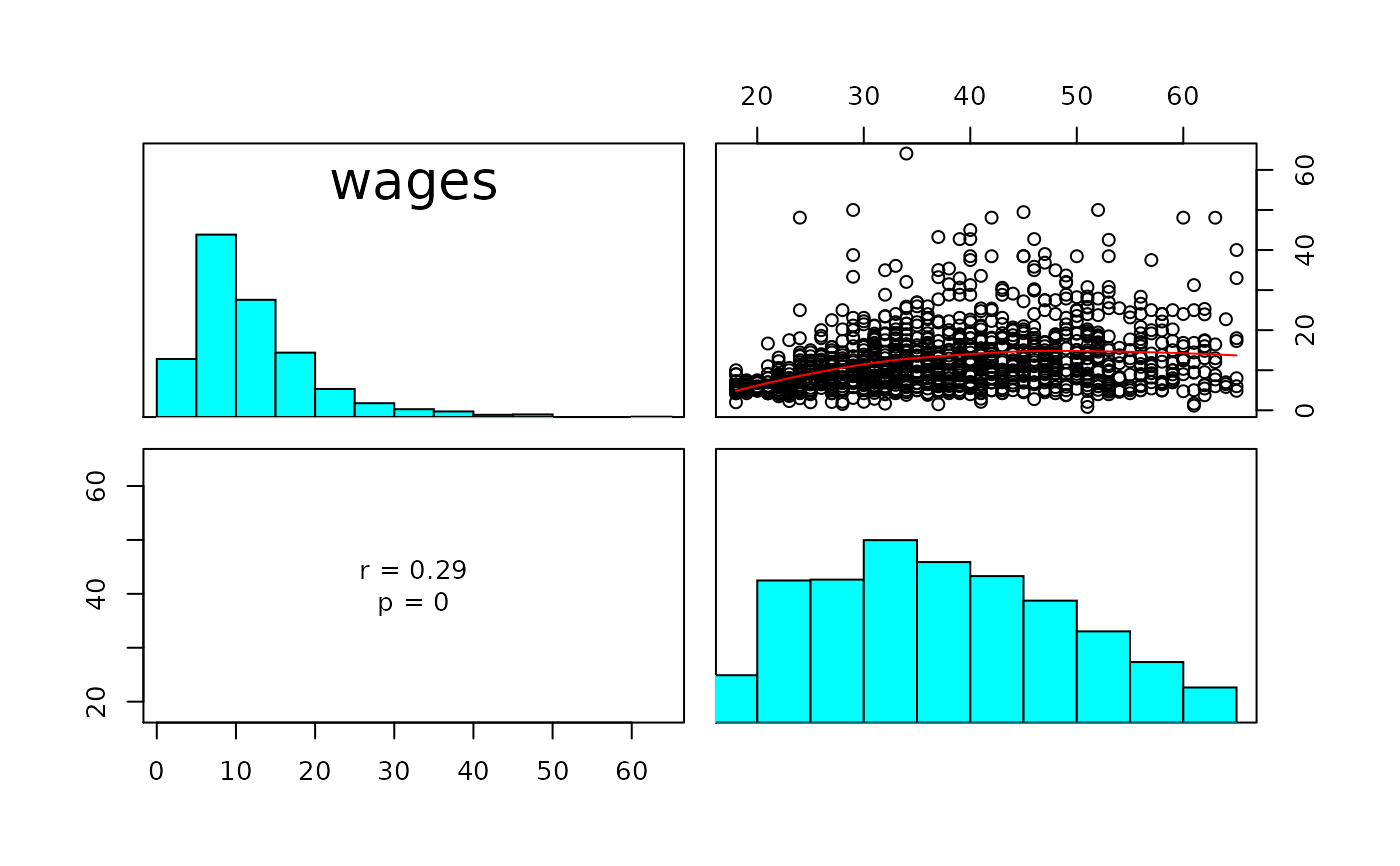
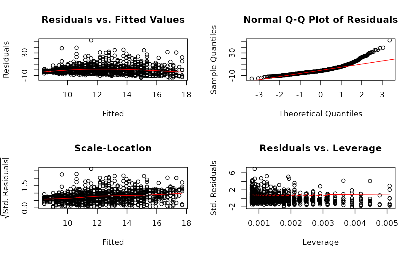
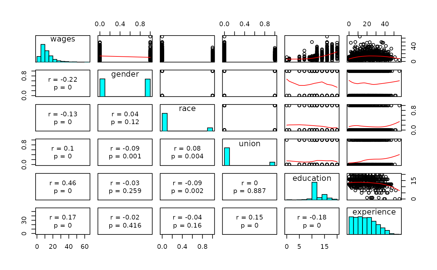
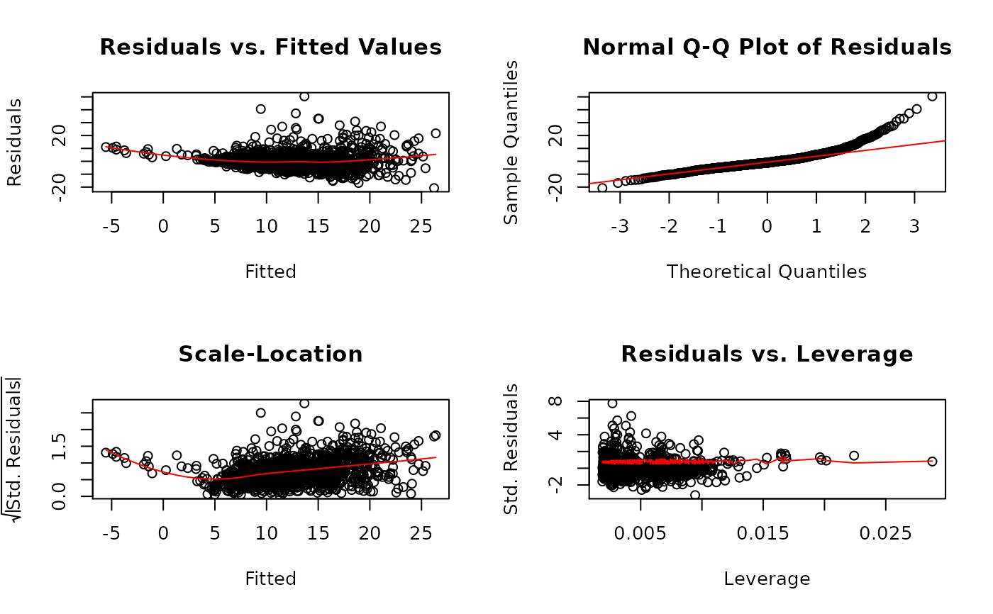
# Simple regression------------------------------------------------
X <- jeksterslabRdatarepo::wages.matrix[["X"]]
X <- X[, c(1, ncol(X))]
y <- jeksterslabRdatarepo::wages.matrix[["y"]]
linreg(X = X, y = y)
#> 
#> Model Assessment:
#>                   Value
#> RSS            73673.13
#> MSE               57.16
#> RMSE               7.56
#> R-squared          0.08
#> Adj. R-squared     0.08
#> 
#> ANOVA Table:
#>         df        SS         MS        F            p
#> Model    1  6636.695 6636.69500 115.9368 6.019852e-26
#> Error 1287 73673.129   57.24408       NA           NA
#> Total 1288 80309.824         NA       NA           NA
#> 
#> Coefficients:
#>               coef         se         t            p
#> Intercept 4.874251 0.72698105  6.704784 3.011026e-11
#> age       0.197486 0.01834111 10.767395 6.019852e-26
#> 
#> Standardized Coefficients:
#> Yuan and Chan 2011 standard errors are used.
#>          coef         se        t           p
#> age 0.2874694 0.02556128 11.24628 4.68231e-28
#> 
#> Confidence Intervals - Regression Coefficients:
#>             ci_0.05    ci_0.5    ci_2.5   ci_97.5   ci_99.5  ci_99.95
#> Intercept 2.4765930 2.9988909 3.4480531 6.3004490 6.7496112 7.2719091
#> age       0.1369951 0.1501723 0.1615042 0.2334678 0.2447997 0.2579769
#> 
#> Confidence Intervals - Standardized Slopes:
#>       ci_0.05    ci_0.5   ci_2.5   ci_97.5   ci_99.5  ci_99.95
#> age 0.2031656 0.2215301 0.237323 0.3376157 0.3534087 0.3717731
#> 
#> Means and Standard Deviations:
#>           Mean       SD
#> wages 12.36585  7.89635
#> age   37.93483 11.49428

# Multiple regression----------------------------------------------
X <- jeksterslabRdatarepo::wages.matrix[["X"]]
# age is removed
X <- X[, -ncol(X)]
linreg(X = X, y = y)
#> 
#> Model Assessment:
#>                   Value
#> RSS            54342.54
#> MSE               42.16
#> RMSE               6.49
#> R-squared          0.32
#> Adj. R-squared     0.32
#> 
#> ANOVA Table:
#>         df       SS         MS        F             p
#> Model    5 25967.28 5193.45611 122.6149 3.453144e-106
#> Error 1283 54342.54   42.35584       NA            NA
#> Total 1288 80309.82         NA       NA            NA
#> 
#> Coefficients:
#>                  coef         se         t            p
#> Intercept  -7.1833382 1.01578786 -7.071691 2.508276e-12
#> gender     -3.0748755 0.36461621 -8.433184 8.939416e-17
#> race       -1.5653133 0.50918754 -3.074139 2.155664e-03
#> union       1.0959758 0.50607809  2.165626 3.052356e-02
#> education   1.3703010 0.06590421 20.792312 5.507605e-83
#> experience  0.1666065 0.01604756 10.382050 2.659960e-24
#> 
#> Standardized Coefficients:
#> Yuan and Chan 2011 standard errors are used.
#>                   coef         se         t            p
#> gender     -0.19477502 0.02282716 -8.532598 3.979462e-17
#> race       -0.07135673 0.02317122 -3.079541 2.117236e-03
#> union       0.05077872 0.02342286  2.167913 3.034867e-02
#> education   0.48829962 0.02113537 23.103429 5.007598e-99
#> experience  0.24607631 0.02330714 10.557981 4.800438e-25
#> 
#> Confidence Intervals - Regression Coefficients:
#>                ci_0.05     ci_0.5     ci_2.5    ci_97.5    ci_99.5   ci_99.95
#> Intercept  -10.5335348 -9.8037324 -9.1761258 -5.1905507 -4.5629441 -3.8331417
#> gender      -4.2774257 -4.0154638 -3.7901849 -2.3595660 -2.1342872 -1.8723252
#> race        -3.2446781 -2.8788475 -2.5642449 -0.5663817 -0.2517792  0.1140514
#> union       -0.5731336 -0.2095371  0.1031443  2.0888072  2.4014886  2.7650852
#> education    1.1529406  1.2002901  1.2410091  1.4995928  1.5403119  1.5876614
#> experience   0.1136797  0.1252092  0.1351242  0.1980889  0.2080039  0.2195334
#> 
#> Confidence Intervals - Standardized Slopes:
#>                ci_0.05       ci_0.5       ci_2.5     ci_97.5    ci_99.5
#> gender     -0.27006189 -0.253661495 -0.239557685 -0.14999235 -0.1358885
#> race       -0.14777833 -0.131130752 -0.116814367 -0.02589909 -0.0115827
#> union      -0.02647282 -0.009644448  0.004827412  0.09673002  0.1112019
#> education   0.41859249  0.433777402  0.446835936  0.52976331  0.5428218
#> experience  0.16920643  0.185951662  0.200352024  0.29180059  0.3062010
#>               ci_99.95
#> gender     -0.11948815
#> race        0.00506488
#> union       0.12803026
#> education   0.55800676
#> experience  0.32294619
#> 
#> Means and Standard Deviations:
#>                  Mean         SD
#> wages      12.3658495  7.8963503
#> gender      0.4972847  0.5001867
#> race        0.1528317  0.3599648
#> union       0.1590380  0.3658535
#> education  13.1450737  2.8138234
#> experience 18.7897595 11.6628366

# Multiple regression----------------------------------------------
# delta standard errors for standardized coefficients
linreg(X = X, y = y, sehatslopeshatprimetype = "delta")
#> 
#> Model Assessment:
#>                   Value
#> RSS            54342.54
#> MSE               42.16
#> RMSE               6.49
#> R-squared          0.32
#> Adj. R-squared     0.32
#> 
#> ANOVA Table:
#>         df       SS         MS        F             p
#> Model    5 25967.28 5193.45611 122.6149 3.453144e-106
#> Error 1283 54342.54   42.35584       NA            NA
#> Total 1288 80309.82         NA       NA            NA
#> 
#> Coefficients:
#>                  coef         se         t            p
#> Intercept  -7.1833382 1.01578786 -7.071691 2.508276e-12
#> gender     -3.0748755 0.36461621 -8.433184 8.939416e-17
#> race       -1.5653133 0.50918754 -3.074139 2.155664e-03
#> union       1.0959758 0.50607809  2.165626 3.052356e-02
#> education   1.3703010 0.06590421 20.792312 5.507605e-83
#> experience  0.1666065 0.01604756 10.382050 2.659960e-24
#> 
#> Standardized Coefficients:
#> Yuan and Chan 2011 standard errors are used.
#>                   coef         se         t            p
#> gender     -0.19477502 0.02282716 -8.532598 3.979462e-17
#> race       -0.07135673 0.02317122 -3.079541 2.117236e-03
#> union       0.05077872 0.02342286  2.167913 3.034867e-02
#> education   0.48829962 0.02113537 23.103429 5.007598e-99
#> experience  0.24607631 0.02330714 10.557981 4.800438e-25
#> 
#> Confidence Intervals - Regression Coefficients:
#>                ci_0.05     ci_0.5     ci_2.5    ci_97.5    ci_99.5   ci_99.95
#> Intercept  -10.5335348 -9.8037324 -9.1761258 -5.1905507 -4.5629441 -3.8331417
#> gender      -4.2774257 -4.0154638 -3.7901849 -2.3595660 -2.1342872 -1.8723252
#> race        -3.2446781 -2.8788475 -2.5642449 -0.5663817 -0.2517792  0.1140514
#> union       -0.5731336 -0.2095371  0.1031443  2.0888072  2.4014886  2.7650852
#> education    1.1529406  1.2002901  1.2410091  1.4995928  1.5403119  1.5876614
#> experience   0.1136797  0.1252092  0.1351242  0.1980889  0.2080039  0.2195334
#> 
#> Confidence Intervals - Standardized Slopes:
#>                ci_0.05       ci_0.5       ci_2.5     ci_97.5    ci_99.5
#> gender     -0.27006189 -0.253661495 -0.239557685 -0.14999235 -0.1358885
#> race       -0.14777833 -0.131130752 -0.116814367 -0.02589909 -0.0115827
#> union      -0.02647282 -0.009644448  0.004827412  0.09673002  0.1112019
#> education   0.41859249  0.433777402  0.446835936  0.52976331  0.5428218
#> experience  0.16920643  0.185951662  0.200352024  0.29180059  0.3062010
#>               ci_99.95
#> gender     -0.11948815
#> race        0.00506488
#> union       0.12803026
#> education   0.55800676
#> experience  0.32294619
#> 
#> Means and Standard Deviations:
#>                  Mean         SD
#> wages      12.3658495  7.8963503
#> gender      0.4972847  0.5001867
#> race        0.1528317  0.3599648
#> union       0.1590380  0.3658535
#> education  13.1450737  2.8138234
#> experience 18.7897595 11.6628366